Introductory examples for esttab
- Basic syntax and usage
- Standard errors, p-values, and summary statistics
- Beta coefficients
- Wide table: coefficients and t-statistics side-by-side
- Numerical formats
- Labels, titles, and notes
- Plain table
- Compressed table
- Significance stars: change symbols and thresholds
- Use with Excel
- Use with Word
- Use with LaTeX
- Non-standard table contents
- Viewing the internal estout call
Basic syntax and usage
esttab is a wrapper for estout. Its syntax is much simpler than that of estout and, by default, it produces publication-style tables that display nicely in Stata's results window. The basic syntax of esttab is:
esttab [ namelist ] [ using filename ] [ , options estout_options ]
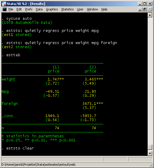
The procedure is to first store a number of models and then apply esttab to these stored estimation sets to compose a regression table. The main difference between esttab and estout is that esttab produces a fully formatted right away. Example:
. sysuse auto
(1978 Automobile Data)
. eststo: quietly regress price weight mpg
(est1 stored)
. eststo: quietly regress price weight mpg foreign
(est2 stored)
. esttab
--------------------------------------------
(1) (2)
price price
--------------------------------------------
weight 1.747** 3.465***
(2.72) (5.49)
mpg -49.51 21.85
(-0.57) (0.29)
foreign 3673.1***
(5.37)
_cons 1946.1 -5853.7
(0.54) (-1.73)
--------------------------------------------
N 74 74
--------------------------------------------
t statistics in parentheses
* p<0.05, ** p<0.01, *** p<0.001
. eststo clear
Note that the dashed lines appear as solid lines in Stata's results window:
Standard errors, p-values, and summary statistics
The default in esttab is to display raw point estimates along with t statistics and to print the number of observations in the table footer. To replace the t-statistics by, e.g., standard errors and add the adjusted R-squared type:
. sysuse auto
(1978 Automobile Data)
. eststo: quietly regress price weight mpg
(est1 stored)
. eststo: quietly regress price weight mpg foreign
(est2 stored)
. esttab, se ar2
--------------------------------------------
(1) (2)
price price
--------------------------------------------
weight 1.747** 3.465***
(0.641) (0.631)
mpg -49.51 21.85
(86.16) (74.22)
foreign 3673.1***
(684.0)
_cons 1946.1 -5853.7
(3597.0) (3377.0)
--------------------------------------------
N 74 74
adj. R-sq 0.273 0.478
--------------------------------------------
Standard errors in parentheses
* p<0.05, ** p<0.01, *** p<0.001
The t-statistics can also be replaced by p-values (p), confidence intervals (ci), or any parameter statistics contained in the estimates (see the aux() option). Further summary statistics options are, for example, pr2 for the pseudo R-squared and bic for Schwarz's information criterion. Moreover, there is a generic scalars() option to include any other scalar statistics contained in the stored estimates. For instance, to print p-values and add the overall F-statistic and information on the degrees of freedom, type:
. esttab, p scalars(F df_m df_r)
--------------------------------------------
(1) (2)
price price
--------------------------------------------
weight 1.747** 3.465***
(0.008) (0.000)
mpg -49.51 21.85
(0.567) (0.769)
foreign 3673.1***
(0.000)
_cons 1946.1 -5853.7
(0.590) (0.087)
--------------------------------------------
N 74 74
F 14.74 23.29
df_m 2 3
df_r 71 70
--------------------------------------------
p-values in parentheses
* p<0.05, ** p<0.01, *** p<0.001
. eststo clear
Beta coefficients
To display beta coefficients and suppress the t-statistics type:
. sysuse auto
(1978 Automobile Data)
. eststo: quietly regress price weight mpg
(est1 stored)
. eststo: quietly regress price weight mpg foreign
(est2 stored)
. esttab, beta not
--------------------------------------------
(1) (2)
price price
--------------------------------------------
weight 0.460** 0.913***
mpg -0.097 0.043
foreign 0.573***
--------------------------------------------
N 74 74
--------------------------------------------
Standardized beta coefficients
* p<0.05, ** p<0.01, *** p<0.001
. eststo clear
Wide table: coefficients and t-statistics side-by-side
The wide option arranges point estimates and t-statistics beside one another instead of beneath one another:
. sysuse auto
(1978 Automobile Data)
. eststo: quietly regress price weight mpg
(est1 stored)
. eststo: quietly regress price weight mpg foreign
(est2 stored)
. esttab, wide
----------------------------------------------------------------------
(1) (2)
price price
----------------------------------------------------------------------
weight 1.747** (2.72) 3.465*** (5.49)
mpg -49.51 (-0.57) 21.85 (0.29)
foreign 3673.1*** (5.37)
_cons 1946.1 (0.54) -5853.7 (-1.73)
----------------------------------------------------------------------
N 74 74
----------------------------------------------------------------------
t statistics in parentheses
* p<0.05, ** p<0.01, *** p<0.001
. eststo clear
Numerical formats
esttab has sensible default settings for numerical display formats. For example, t-statistics are printed using two decimal places and R-squared measures are printed using three decimal places. For point estimates and, for example, standard errors an adaptive display format is used where the number of displayed decimal places depends on the scale of the statistic to be printed (the default format is a3; see below).
The format applied to a certain statistic can be changed by adding the appropriate display format specification in parentheses. For example, to increase precision for the point estimates and display p-values and the R-squared using four decimal places, type:
. sysuse auto
(1978 Automobile Data)
. eststo: quietly regress price weight mpg
(est1 stored)
. eststo: quietly regress price weight mpg foreign
(est2 stored)
. esttab, b(a6) p(4) r2(4) nostar wide
----------------------------------------------------------------
(1) (2)
price price
----------------------------------------------------------------
weight 1.746559 (0.0081) 3.464706 (0.0000)
mpg -49.51222 (0.5673) 21.85360 (0.7693)
foreign 3673.060 (0.0000)
_cons 1946.069 (0.5902) -5853.696 (0.0874)
----------------------------------------------------------------
N 74 74
R-sq 0.2934 0.4996
----------------------------------------------------------------
p-values in parentheses
. eststo clear
Available formats are official Stata's display formats, such as %9.0g or %8.2f (see help format). Alternatively, as is illustrated in the example above, a fixed format can be requested by specifying a single integer indicating the desired number of decimal places. Furthermore, an adaptive format a# may be specified, where # determines the minimum number of "significant digits" to be printed (# should be in {1,2,...,9}) (see the Numerical formats section in the help file).
Labels, titles, and notes
To use variable labels and add some titles and notes, e.g., type:
. sysuse auto
(1978 Automobile Data)
. eststo: quietly regress price weight mpg
(est1 stored)
. eststo: quietly regress price weight mpg foreign
(est2 stored)
. esttab, label ///
> title(This is a regression table) ///
> nonumbers mtitles("Model A" "Model B") ///
> addnote("Source: auto.dta")
This is a regression table
----------------------------------------------------
Model A Model B
----------------------------------------------------
Weight (lbs.) 1.747** 3.465***
(2.72) (5.49)
Mileage (mpg) -49.51 21.85
(-0.57) (0.29)
Car type 3673.1***
(5.37)
Constant 1946.1 -5853.7
(0.54) (-1.73)
----------------------------------------------------
Observations 74 74
----------------------------------------------------
t statistics in parentheses
Source: auto.dta
* p<0.05, ** p<0.01, *** p<0.001
. eststo clear
The label option supports factor variables and interactions in Stata 11 or newer:
. sysuse auto
(1978 Automobile Data)
. eststo: quietly regress price mpg i.foreign
(est1 stored)
. eststo: quietly regress price c.mpg##i.foreign
(est2 stored)
. esttab, varwidth(25)
---------------------------------------------------------
(1) (2)
price price
---------------------------------------------------------
mpg -294.2*** -329.3***
(-5.28) (-4.39)
0.foreign 0 0
(.) (.)
1.foreign 1767.3* -13.59
(2.52) (-0.01)
0.foreign#c.mpg 0
(.)
1.foreign#c.mpg 78.89
(0.70)
_cons 11905.4*** 12600.5***
(10.28) (8.25)
---------------------------------------------------------
N 74 74
---------------------------------------------------------
t statistics in parentheses
* p<0.05, ** p<0.01, *** p<0.001
. esttab, varwidth(25) label
---------------------------------------------------------
(1) (2)
Price Price
---------------------------------------------------------
Mileage (mpg) -294.2*** -329.3***
(-5.28) (-4.39)
Domestic 0 0
(.) (.)
Foreign 1767.3* -13.59
(2.52) (-0.01)
Domestic # Mileage (mpg) 0
(.)
Foreign # Mileage (mpg) 78.89
(0.70)
Constant 11905.4*** 12600.5***
(10.28) (8.25)
---------------------------------------------------------
Observations 74 74
---------------------------------------------------------
t statistics in parentheses
* p<0.05, ** p<0.01, *** p<0.001
. esttab, varwidth(25) label nobaselevels interaction(" X ")
---------------------------------------------------------
(1) (2)
Price Price
---------------------------------------------------------
Mileage (mpg) -294.2*** -329.3***
(-5.28) (-4.39)
Foreign 1767.3* -13.59
(2.52) (-0.01)
Foreign X Mileage (mpg) 78.89
(0.70)
Constant 11905.4*** 12600.5***
(10.28) (8.25)
---------------------------------------------------------
Observations 74 74
---------------------------------------------------------
t statistics in parentheses
* p<0.05, ** p<0.01, *** p<0.001
. eststo clear
Plain table
The plain option produces a minimally formatted table with all display formats set to Stata's %9.0g quasi-standard:
. sysuse auto
(1978 Automobile Data)
. eststo: quietly regress price weight mpg
(est1 stored)
. eststo: quietly regress price weight mpg foreign
(est2 stored)
. esttab, plain
est1 est2
b/t b/t
weight 1.746559 3.464706
2.723238 5.493003
mpg -49.51222 21.8536
-.5746808 .2944391
foreign 3673.06
5.370142
_cons 1946.069 -5853.696
.541018 -1.733408
N 74 74
. eststo clear
Compressed table
The compress option reduces horizontal spacing to fit more models on screen without line breaking:
. sysuse auto
(1978 Automobile Data)
. eststo: quietly regress price weight
(est1 stored)
. eststo: quietly regress price weight mpg
(est2 stored)
. eststo: quietly regress price weight mpg foreign
(est3 stored)
. eststo: quietly regress price weight mpg foreign displacement
(est4 stored)
. esttab, compress
--------------------------------------------------------------
(1) (2) (3) (4)
price price price price
--------------------------------------------------------------
weight 2.044*** 1.747** 3.465*** 2.458**
(5.42) (2.72) (5.49) (2.82)
mpg -49.51 21.85 19.08
(-0.57) (0.29) (0.26)
foreign 3673.1*** 3930.2***
(5.37) (5.67)
displace~t 10.22
(1.65)
_cons -6.707 1946.1 -5853.7 -4846.8
(-0.01) (0.54) (-1.73) (-1.43)
--------------------------------------------------------------
N 74 74 74 74
--------------------------------------------------------------
t statistics in parentheses
* p<0.05, ** p<0.01, *** p<0.001
. eststo clear
Significance stars: change symbols and thresholds
The default symbols and thresholds are for the "significance stars" are: * for p<.05, ** for p<.01, and *** for p<.001. To use + for p<.10 and * for p<.05, for example, type:
. sysuse auto
(1978 Automobile Data)
. eststo: quietly regress price weight mpg
(est1 stored)
. eststo: quietly regress price weight mpg foreign
(est2 stored)
. esttab, star(+ 0.10 * 0.05)
----------------------------------------
(1) (2)
price price
----------------------------------------
weight 1.747* 3.465*
(2.72) (5.49)
mpg -49.51 21.85
(-0.57) (0.29)
foreign 3673.1*
(5.37)
_cons 1946.1 -5853.7+
(0.54) (-1.73)
----------------------------------------
N 74 74
----------------------------------------
t statistics in parentheses
+ p<0.10, * p<0.05
. eststo clear
Use the nostar option suppresses the significance stars.
Use with Excel
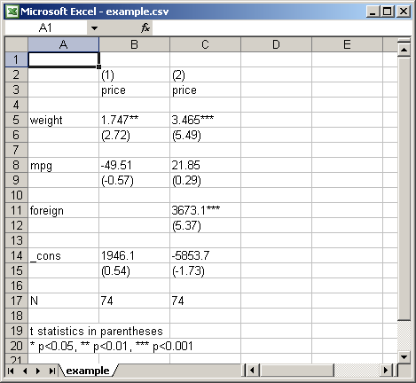
To produce a table for use with Excel, specify an output filename and apply the csv format (or the scsv format depending on the language version of Excel). For example:
. sysuse auto (1978 Automobile Data) . eststo: quietly regress price weight mpg (est1 stored) . eststo: quietly regress price weight mpg foreign (est2 stored) . esttab using example.csv (output written to example.csv)
A click on "example.csv" in Stata's results window will launch Excel and display the file:
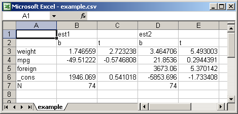
Depending on whether the plain option is specified or not, esttab uses two different variants of the CSV format. By default, that is, if plain is omitted, the contents of the table cells are enclosed in double quotes preceded by an equal sign (i.e. ="..."). This prevents Excel from trying to interpret the contents of the cells and, therefore, preserves formatting elements such as parentheses around t-statistics. One drawback of this approach is, however, that the displayed numbers cannot directly be used for further calculations in Excel. Hence, if the purpose of exporting the estimates is to do additional computations in Excel, specify the plain option. In this case, the table cells are enclosed in double quotes without the equal sign, and Excel will interpret the contents as numbers. Example:
. esttab using example.csv, replace wide plain (output written to example.csv) . eststo clear
Result:
Use with Word
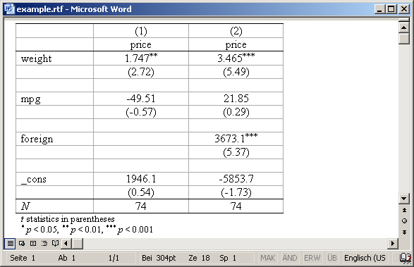
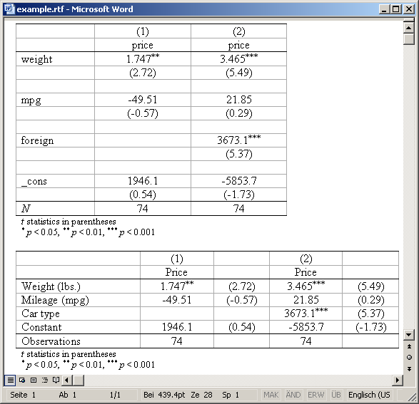
To produce a table for use with Word, specify an output filename with an .rtf suffix or apply the rtf format:
. sysuse auto (1978 Automobile Data) . eststo: quietly regress price weight mpg (est1 stored) . eststo: quietly regress price weight mpg foreign (est2 stored) . esttab using example.rtf (output written to example.rtf)
Result:
Appending is possible. Furthermore, varwidth() and modelwidth() may be used to change the column widths (the scale is about 1/12 inch). Example
. esttab using example.rtf, append wide label modelwidth(8) (output written to example.rtf)
Result:
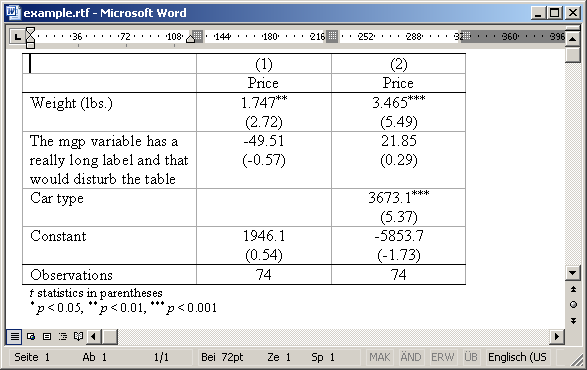
Another very useful feature is the onecell option that causes the point estimates and t statistics (or standard errors, etc.) to be placed beneath one another in the same table cell:
. lab var mpg "The mgp variable has a really long label and that would disturb > the table" . esttab using example.rtf, replace label nogap onecell (output written to example.rtf)
Result:
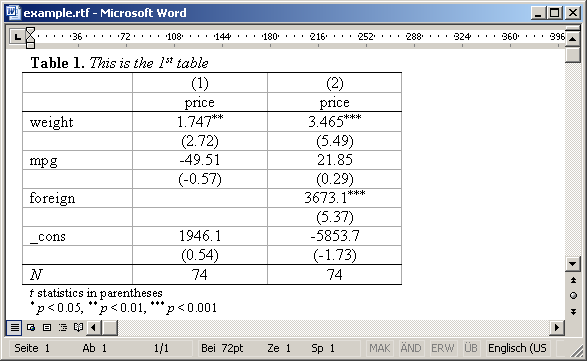
If you know a bit RTF you can also include RTF commands to achieve specific effects, although you have to be careful not to break the document (most importantly, do not introduce unmatched curly braces). Useful are, for example, "{\b ...}" for boldface and "{\i ...}" for italics. A very helpful reference is the "RTF Pocket Guide" by Sean M. Burke (O'Reilly). Example
. esttab using example.rtf, replace nogaps ///
> title({\b Table 1.} {\i This is the 1{\super st} table})
(output written to example.rtf)
Result:
Use with LaTeX
To create a table to be included in a LaTeX document, type:
. sysuse auto
(1978 Automobile Data)
. eststo: quietly regress price weight mpg
(est1 stored)
. eststo: quietly regress price weight mpg foreign
(est2 stored)
. esttab using example.tex, label nostar ///
> title(Regression table\label{tab1})
(output written to example.tex)
TeXifying a document containing
\documentclass{article}
\begin{document}
\input{example.tex}
\end{document}
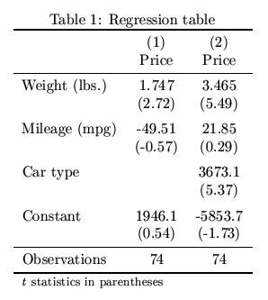
then produces the following result:
Note that esttab automatically initializes the tabular environment and, if title() is specified, sets the table as a float object. Use the fragment option if you prefer to hard-code the table's environment and have esttab just produce the table rows.
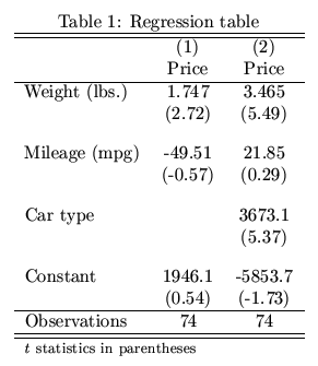
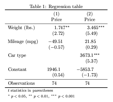
The table above looks alright, but a better result is achieved by specifying the booktabs option and loading LaTeX's booktabs package in the document preamble:
. esttab using example.tex, label nostar replace booktabs ///
> title(Regression table\label{tab1})
(output written to example.tex)
Result:
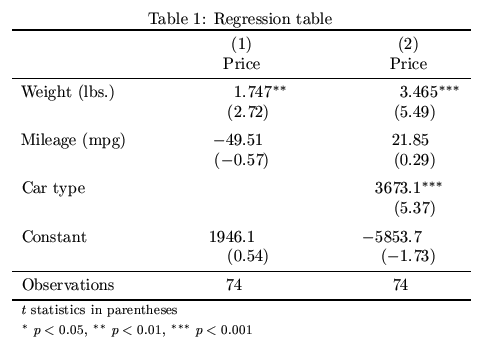
A further improvement is to load LaTeX's dcolumn package and format the columns using the D column specifier:
. esttab using example.tex, label replace booktabs ///
> alignment(D{.}{.}{-1}) ///
> title(Regression table\label{tab1})
(output written to example.tex)
Result:
Last but not least, it might be reasonable to space the table out to a certain width:
. esttab using example.tex, label replace booktabs ///
> alignment(D{.}{.}{-1}) width(0.8\hsize) ///
> title(Regression table\label{tab1})
(output written to example.tex)
. eststo clear
Result:
Non-standard table contents
Sometimes it is necessary to include parameter statistics in a table for which no predefined option exists in esttab. Once the statistics are are stored in an e()-matrix, they can be displayed using the main() option (replacing the point-estimates) or the aux() option (replacing the t-statistics). For example, to include variance inflation factors instead of t-statistics after regress, you could type:
. sysuse auto
(1978 Automobile Data)
. quietly regress price weight mpg foreign
. estadd vif
Variable | VIF 1/VIF
-------------+----------------------
weight | 3.86 0.258809
mpg | 2.96 0.337297
foreign | 1.59 0.627761
-------------+----------------------
Mean VIF | 2.81
added matrix:
e(vif) : 1 x 4
. esttab, aux(vif 2) wide nopar
-----------------------------------------
(1)
price
-----------------------------------------
weight 3.465*** 3.86
mpg 21.85 2.96
foreign 3673.1*** 1.59
_cons -5853.7
-----------------------------------------
N 74
-----------------------------------------
vif in second column
* p<0.05, ** p<0.01, *** p<0.001
(Note: The second argument in aux() specifies the display format.)
However, if you want to include more than two kinds of parameter statistics, you have to switch to estout syntax and make use of the cells() option. All estout options are allowed in esttab, but you have to be aware that the specified estout options will take precedence over esttab's own options. For example, specifying cells() disables b(), beta(), main(), t(), abs, not, se(), p(), ci(), aux(), star, staraux, wide, onecell, parentheses, and brackets. In the following example the cells() option is used to print point estimates, t statistics, and variance inflation factors in one table:
. sysuse auto
(1978 Automobile Data)
. quietly regress price weight mpg foreign
. estadd vif
Variable | VIF 1/VIF
-------------+----------------------
weight | 3.86 0.258809
mpg | 2.96 0.337297
foreign | 1.59 0.627761
-------------+----------------------
Mean VIF | 2.81
added matrix:
e(vif) : 1 x 4
. esttab, cells("b(fmt(a3) star) vif(fmt(2))" t(par fmt(2)))
-----------------------------------------
(1)
price
b/t vif
-----------------------------------------
weight 3.465*** 3.86
(5.49)
mpg 21.85 2.96
(0.29)
foreign 3673.1*** 1.59
(5.37)
_cons -5853.7
(-1.73)
-----------------------------------------
N 74
-----------------------------------------
Similarly, for a complicated summary statistics section in the table footer you might have to use estout's stats() option (which overwrites esttab options such as r2(), ar2(), pr2(), aic(), bic(), scalars(), sfmt(), noobs, and obslast.)
Viewing the internal estout call
Sometimes, an approach is to use esttab to assemble a basic table and then hand-edit and re-run the estout call. The call can be made visible by the noisily option and is also returned in r(cmdline). Example:
. sysuse auto
(1978 Automobile Data)
. eststo: quietly regress price weight mpg
(est1 stored)
. eststo: quietly regress price weight mpg foreign
(est2 stored)
. esttab, noisily notype
estout ,
cells(b(fmt(a3) star) t(fmt(2) par("{ralign @modelwidth:{txt:(}" "{txt:)}}")))
stats(N, fmt(%18.0g) labels(`"N"'))
starlevels(* 0.05 ** 0.01 *** 0.001)
varwidth(12)
modelwidth(12)
abbrev
delimiter(" ")
smcltags
prehead(`"{hline @width}"')
posthead("{hline @width}")
prefoot("{hline @width}")
postfoot(`"{hline @width}"' `"t statistics in parentheses"' `"@starlegend"')
varlabels(, end("" "") nolast)
mlabels(, depvar)
numbers
collabels(none)
eqlabels(, begin("{hline @width}" "") nofirst)
interaction(" # ")
notype
level(95)
style(esttab)
. return list
scalars:
r(nmodels) = 2
r(ccols) = 3
macros:
r(names) : "est1 est2"
r(m2_depname) : "price"
r(m1_depname) : "price"
r(cmdline) : "estout , cells(b(fmt(a3) star) t(fmt(2) par("{ral.."
matrices:
r(coefs) : 4 x 6
r(stats) : 1 x 2
. eststo clear
(notype is specified in this example to suppress the display of the table.)